R-package 'Luminescence'

This webpage has been abandoned. Please visit our new package webpage: 
http://www.r-luminescence.de

 

Developer Team

• Christoph Burow (University of Cologne)
• Michael Dietze (TU Dresden)
• Manfred Fischer (University of Bayreuth)
• Margret C. Fuchs (TU Bergakademie Freiberg)
• Christoph Schmidt (University of Bayreuth)
• Sebastian Kreutzer (JLU Giessen)

Latest package version on CRAN: 0.2.4

Next package update: 0.3, mid of July 2013

Package maintainer: Sebastian Kreutzer (research group Prof. Dr. Markus Fuchs)

Citation:

citation("Luminescence") 

## To cite package 'Luminescence' in publications use: ## ## Kreutzer S, Schmidt C, Fuchs MC, Dietze M, Fischer M, Burow C and ## Fuchs M (2013). _Luminescence: Package for Luminescence Dating ## data analysis_. R package version 0.2.4, <URL: ## http://CRAN.R-project.org/package=Luminescence>. ## ## Kreutzer S, Schmidt C, Fuchs MC, Dietze M, Fischer M and Fuchs M ## (2012). "Introducing an R package for luminescence dating ## analysis." _Ancient TL_, *30*, pp. 1-8. 

Tutorials

• Dietze, M., Fuchs, M.C., Kreutzer, S., 2013. From bin-files to De-distributions. R Luminesccence Package Tutorial.
  • Tutorial as HTML (EN) in a ZIP folder

Workshops

2012

• 26th October 2012, 6.00 to 8.00 pm (German LED Mannheim; location: C4,8; 4th floor)
  • Tutorial as PDF (EN)
  • Tutorial as PDF (DE)

Package Overview

Using minerals in sediments as natural dosimeters allows to date the time of their last daylight exposure or the last heating event. This dating technique is usually referred as optically stimulated luminescence (OSL) or thermal luminescence (TL) dating. The luminescence dating technique has been greatly advanced since the experimental beginnings and is now a standard technique to provide numerical ages to the geoscientific and archaeological community.

Analysis of measurement data is usually accomplished using proprietary software, bundled with the luminescence measurement device (e.g. Risø reader). Yet, to allow flexible analysis of new measurement protocols, provide a fully open source code of the analysis procedures which may be edited and modified by the user, and – perhaps most important – to provide high-quality graphical and numerical data presentation a different approach needs to be introduced.

R and R-packages

R is an open-source software. Along with freely available user interfaces such as RStudio or RKWard, the underpinned command-line structure is greatly aided by window- and menu-based user interaction. R provides a powerful, flexible and universal tool for extensive data analysis and visualisation. There are many excellent webpages (e.g. http://rwiki.sciviews.org) that may help to find an easy way into the R groove.

The basic functionality of R can be greatly extended by using additional R-packages, collections of functions, designed for special tasks. One such task may be the evaluation of luminescence measurement data.

Contents of the package 'Luminescence'

The package 'Luminescence' comprises a series of functions that allow to import, analyse, evaluate and visualise luminescence measurement data. The package is provided under General Public License (GPL) license and, accordingly, freely available to everyone.

Functions bundled with the recent version of the package

Name	Description
Analyse_SAR.OSLdata()	Analyse SAR CW-OSL measurements
Calc_CentralDose()	Apply the central age model (CAM) after Galbraith et al. (1999) to a given De distribution
Calc_CommonDose()	Apply the (un-)logged common age model after Galbraith et al. (1999) to a given De distribution
Calc_FadingCorr()	Applying a fading correction according to Huntley & Lamothe (2001) for a given age and a given g-value
Calc_FiniteMixture()	Apply the finite mixture model (FMM) after Galbraith (2005) to a given De distribution
Calc_FuchsLang2001()	Calculate De applying the method of Fuchs and Lang (2001)
Calc_MinDose3()	Apply the (un-)logged three parameter minimum age model (MAM 3) after Galbraith et al. (1999) to a given De distribution
Calc_MinDose4()	Apply the (un-)logged three parameter minimum age model (MAM 4) after Galbraith et al. (1999) to a given De distribution
Calc_OSLLxTxRatio()	Calculate Lx/Tx ratio for a given set of OSL curves
CW2pHMi()	Transform a CW-OSL curve into a pHM-OSL curve via interpolation under hyperbolic modulation conditions
CW2pLM()	Transform a CW-OSL curve into a pseudo-LM (pLM) curve (e.g. Bulur, 2000)
CW2pLMi()	Transform a CW-OSL curve into a pLM-OSL curve via interpolation under linear modulation conditions
CW2pPMi()	Transform a CW-OSL curve into a pPM-OSL curve via interpolation under parabolic modulation conditions
fit_CWCurve()	Nonlinear Least Squares Fit for CW-OSL curves
fit_LMCurve()	Non-linear Least Squares (NLS) fit for LM-OSL curves
plot_BINfileData()	Plot single luminescence curves from a BIN-file object (readBIN2R())
plot_KDE()	Plot a kernel density estimate (KDE), sorted values with associated errors and statistical measures
plot_GrowthCurve()	Fit and plot a growth curve for luminescence data
plot_Histogram()	Plot a histogram with a separate error plot
plot_RadialPlot()	Plot a Galbraith's radial plot
readBIN2R()	Import Risø BIN-file into R
Second2Gray()	Converting values from seconds (s) to Gray (Gy)

Obtaining and using the package, support

Using the R-package Luminescence is quite simple and requires three basic steps:

1. Download and install R and, preferably, RStudio: http://cran.r-project.org/, http://rstudio.org
2. Install the package (necessary only once): install.packages(“Luminescence”, dependencies=TRUE)
3. Load the package (once per session): library(Luminescence)

The most important message

The package lives and prospers from nothing else but the contributions of ideas, critics and time to it. Please help us to improve the package, to fix bugs, to enhance existing and add new functions, to make it more user friendly, to make it more usable for the community and – most important – to use it. Your contribution may be as simple as writing an email to mention present shortcomings, suggest solutions or ideas of new functionality. It is easy and takes only a moment, but it would help us considerably to bring the package forward.

Some examples

Import a BIN-file

The function readBIN2R() parses the entire content of a BIN-file, generated by the Risø Sequence Editor (file versions 3.x and 4.x), and writes it into an R object with two slots.

D <- readBIN2R("data.BIN")

## [readBIN2R.R] ## data.BIN ## |==========================| 100% ## 744 records have been read successfully! 

The imported data set (written to the variable D) reveals two slots. METADATA and DATA two slots.

• METADATA contains all information on the measurement and corresponds to what is shown when using the display Information options in the Analyst software.
• DATA contains the raw measured count data of the luminescence reader.

Showing the object itself yields a summary of the imported file (in the following example the example data provided with the package is used)

library(Luminescence) 

## Loading required package: shape 

## Welcome to the R package Luminescence version 0.2.3 [Built: 2013-03-29 ## 17:03:44 UTC] 

data(ExampleData.BINfileData) D <- BINfileData D 

## ## Risoe.BINfileData Object ## Version: 03 ## Object Date: 060920 ## User: Default ## System ID: 0 ## Overall Records: 720 ## Records Type: TL=360; OSL=336; IRSL=24; ## Position Range: 1 : 24 ## Run Range: 1 : 8 ## Set Range: 2 : 6 

Analyse SAR OSL data

The function Analyse_SAR.OSLdata() returns a summarising graphical output, containing Ln/Lx-curves, Tn/Tx-curves, cutheat-TL-curves as well as IRSL-curves. The graphical output may be used for as it stands or for copy-and-paste to conduct further modifications.

SAR <- Analyse_SAR.OSLdata(input.data = D, signal.integral = c(1:5), background.integral = c(900:1000), position = c(1:1), output.plot = TRUE)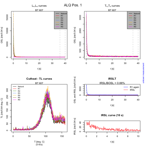 

## ## [Analyse_OSLCurves.R] >> Figure for position 1 produced. 

The function provides further parameters which may be used as rejection criteria.

SAR$RejectionCriteria 

## R5/R1 Recuperation IRSL_BOSL ## [1,] 1.046 0.0039 0.0088 

Constructing growth curves

The function plot_GrowthCurve() performs a fit of the measured De values by a series of possible, user-defined functions and returns numerical (e.g. natural De and model parameters) as well as graphical results:

library(Luminescence) data(ExampleData.LxTxData) plot_GrowthCurve(LxTxData) 

## [plot_GrowthCurve.R] >> D01 = 1766.07 

## $De ## De De.Error D01 D02 Fit ## 1 1738 26.69 1766 NA EXP ## ## $Fit ## Nonlinear regression model ## model: y ~ fit.functionEXP(a, b, c, x) ## data: data ## a b c ## 6.81 1766.07 5.05 ## weighted residual sum-of-squares: 0.000427 ## ## Algorithm "port", convergence message: relative convergence (4) 

Data visualisation

CW to pseudo-LM transformation for curve visualisation

library(Luminescence) ## load data data(ExampleData.CW_OSL_Curve) values <- CW_Curve.BosWallinga2012 ## open plot area plot(NA, NA, xlim = c(0.001, 10), ylim = c(0, 8000), ylab = "pseudo OSL (cts/0.01 s)", xlab = "t [s]", log = "x", main = "Fig. 4 - Bos & Wallinga (2012)", ) values.t <- CW2pLMi(values, P = 1/20) lines(values[1:length(values.t[, 1]), 1], CW2pLMi(values, P = 1/20)[, 2], col = "red", lwd = 1.3) text(0.03, 4500, "LM", col = "red", cex = 0.8) values.t <- CW2pHMi(values, delta = 40) lines(values[1:length(values.t[, 1]), 1], CW2pHMi(values, delta = 40)[, 2], col = "black", lwd = 1.3) text(0.005, 3000, "HM", cex = 0.8) values.t <- CW2pPMi(values, P = 1/10) 

## Warning: t' is beyond the time resolution. Only two data points have been ## extrapolated, the first 3 points have been set to 0! 

lines(values[1:length(values.t[, 1]), 1], CW2pPMi(values, P = 1/10)[, 2], col = "blue", lwd = 1.3) 

## Warning: t' is beyond the time resolution. Only two data points have been ## extrapolated, the first 3 points have been set to 0! 

text(0.5, 6500, "PM", col = "blue", cex = 0.8)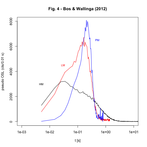 

De values

library(Luminescence) data(ExampleData.DeValues) ## convert values to from seconds to Gray ExampleData.DeValues <- Second2Gray(ExampleData.DeValues, c(0.1, 0.001)) 

Histogram

plot_Histogram(ExampleData.DeValues, xlab = "De [Gy]")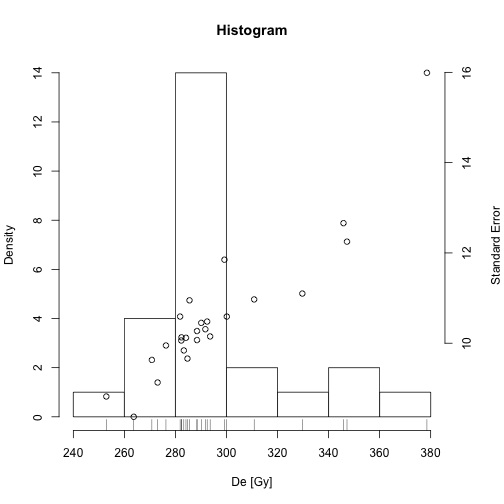 

De distribution with a kernel density estimate (KDE)

plot_KDE(ExampleData.DeValues, distribution.parameters = c("qr", "kdemax"), summary = c("n", "mean", "median", "kdemax", "serel", "sdrel", "sdabs", "seabs"))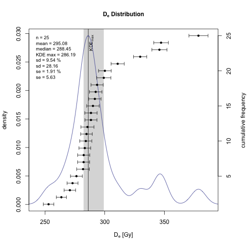 

Galbraith's radial plot

plot_RadialPlot(ExampleData.DeValues, zscale.log = TRUE, zaxis.scale = seq(225, 425, by = 50)) 

## Error: Nicht-numerisches Argument für mathematische Funktion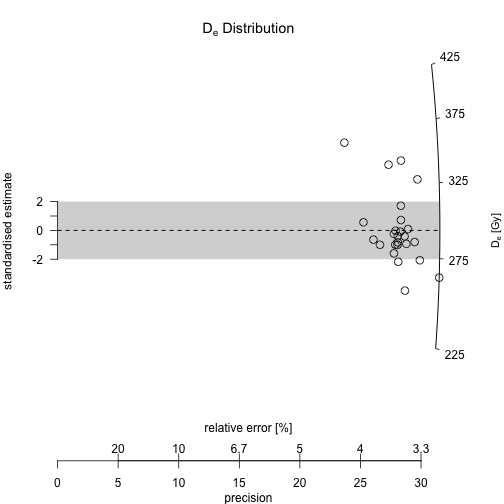 

Signal component stripping (signal deconvolution)

For component stripping the functions fit_CWCurve() (CW-OSL data) or fit_LMCurve() (LM-OSL data) can be used. The function fit_LMCurve() performs fitting of measurement data, following the linear modulation OSL approach (LM-OSL: Bulur, 1996). Several options are provided to take care of signal decomposition and background treatment. The function returns both, graphical and numeric output. The latter may be used for further calculations.

library(Luminescence) data(ExampleData.FittingLM) FLM <- fit_LMCurve(values = values.curve, n.components = 3, log_scale = "x") 

## ## [fit_LMCurve.R] ## ## Fitting was done using a 3-component function: ## ## Im1 Im2 Im3 xm1 xm2 xm3 ## 202.77 367.30 639.21 56.18 1449.72 7878.25 ## ## (equation used for fitting according Kitis & Pagonis, 2008) ## ------------------------------------------------------------------------------ ## (1) Corresponding values according the equation in Bulur, 1996 for b and n0: ## ## b1 = 1.267e+00 +/- NA ## n01 = 1.878e+04 +/- NA ## ## b2 = 1.903e-03 +/- NA ## n02 = 8.779e+05 +/- NA ## ## b3 = 6.445e-05 +/- NA ## n03 = 8.303e+06 +/- NA ## ## cs from component1 = 1.488e-17 cm^2 >> relative: 1 ## cs from component2 = 2.234e-20 cm^2 >> relative: 0.0015 ## cs from component3 = 7.566e-22 cm^2 >> relative: 1e-04 ## ## (stimulation intensity value used for calculation: 8.518e+16 1/s 1/cm^2) ## (errors quoted as 1-sigma uncertainties) ## ------------------------------------------------------------------------------ ## ## pseudo-R^2 = 0.9557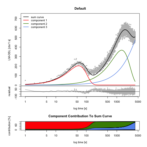 

References

Bos, A.J.J., Wallinga, J., 2012. How to visualize quartz OSL signal components. Radiation Measurements, 47, 752-758. http://dx.doi.org/10.1016/j.radmeas.2012.01.013

Bulur, E., 1996. An Alternative Technique For Optically Stimulated Luminescence (OSL) Experiment. Radiation Measurements 26, 701–709. http://dx.doi.org/10.1016/S1350-4487(97)82884-3

Bulur, E., 2000. A simple transformation for converting CW-OSL curves to LM-OSL curves. Radiation Measurements 32, 141–145. http://dx.doi.org/10.1016/S1350-4487(99)00247-4

Duller, G.A.T., 2007. Analyst. PDF

Fuchs, M., Lang, A., 2001. OSL dating of coarse-grain fluvial quartz using single-aliquot protocols on sediments from NE Peloponnese, Greece. Quaternary Science Reviews 20, 783–787. http://dx.doi.org/10.1016/S0277-3791(00)00040-8

Galbraith, R.F. & Laslett, G.M., 1993. Statistical models for mixed fission track ages. Nuclear Tracks Radiation Measurements, 4, 459-470. http://dx.doi.org/10.1016/1359-0189(93)90185-C

Galbraith, R.F., Roberts, R.G., Laslett, G.M., Yoshida, H. & Olley, J.M., 1999. Optical dating of single grains of quartz from Jinmium rock shelter, northern Australia. Part I: experimental design and statistical models. Archaeometry, 41, 339-364. http://dx.doi.org/10.1111/j.1475-4754.1999.tb00987.x

Galbraith, R.F., 2005. Statistics for Fission Track Analysis, Chapman & Hall/CRC, Boca Raton.

Galbraith, R.F. & Roberts, R.G., 2012. Statistical aspects of equivalent dose and error calculation and display in OSL dating: An overview and some recommendations. Quaternary Geochronology, 11, 1-27.http://dx.doi.org/10.1016/j.quageo.2012.04.020

Huntley, D.J., Lamothe, M., 2001. Ubiquity of anomalous fading in K-feldspars and the measurement and correction for it in optical dating. Canadian Journal of Earth Sciences 38, 1093–1106. http://dx.doi.org/10.1139/e01-013

Kreutzer, S., Schmidt, C., Fuchs, M.C., Dietze, M., Fischer, M., Fuchs, M., 2012. Introducing an R package for luminescence dating analysis. Ancient TL 30, 1–8. Journal Page